Here is a well-structured README.md for your Heated Pipe System with Heat Loss project, including key visuals and explanations:

---

Heated Pipe System with Heat Loss

A tutorial on regulating the outlet temperature of a 450-meter heat pipe near its boiling point, comparing PI, MPC, and Reinforcement Learning control strategies.

---

📌 Overview

This project demonstrates how to regulate the outlet temperature of a 450-meter heat pipe loop for bacteria decontamination, ensuring:

• Outlet temperature > 85°C

• Inlet temperature < 95°C

• Heating rate of 2°C/min

• No steam formation

The system is modeled, simulated, and controlled using three approaches: PI control, Model Predictive Control (MPC), and Reinforcement Learning (RL).

---

🔍 System Description

Physical Setup

• A 450-meter circular pipe with continuous water flow.

• A heater at the entrance provides constant power.

• Water loses heat to the environment via convection.

• The water returns to the heater, creating a closed loop.

Challenges

• Stair-like temperature behavior due to water recirculation.

• Significant delay (~12 min) between input and output.

• Coupling between inlet and outlet temperatures.

• Security constraints: Avoid boiling water or steam.

---

📊 System Modeling

Physical Model

The temperature evolution is governed by the PDE:

\[ \frac{\partial T}{\partial t} + u \frac{\partial T}{\partial x} = -\frac{h P_{\text{pipe}}}{\rho S c_p} \left[ T(x, t) - T_{\text{ext}} \right] \]

Simulation

• The pipe is divided into segments.

• Each segment’s temperature is updated based on neighbors and the environment.

• The heater injects warmth, and the animation shows heat propagation.

---

🎛️ Control Strategies

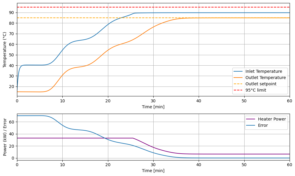
1. PI Control (Proportional-Integral)

• Equation:

\[ u(t) = K_p \, e(t) + K_i \int_0^t e(\tau) \, d\tau \]

• Gain scheduling ensures inlet temperature stays below 95°C.

• Performance: Excellent for constant setpoint tracking.

---

2. Model Predictive Control (MPC)

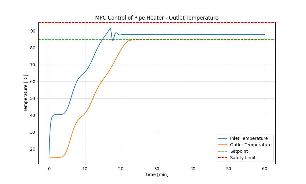
• Objective: Minimize tracking error and input usage over a prediction horizon.

• Constraints: Inlet/outlet temperatures ≤ 95°C, power ≤ 33 kW.

• Advantage: Handles constraints inherently.

---

3. Reinforcement Learning (RL)

• Environment: Heater power as action, temperatures as observations.

• Reward: Balances setpoint tracking, smooth control, energy usage, and safety.

• Algorithm: Soft Actor-Critic (SAC).

• Performance: Struggles with precise tracking but is flexible.

---

📈 Comparison & Conclusion

Criteria	PI Control	MPC	RL
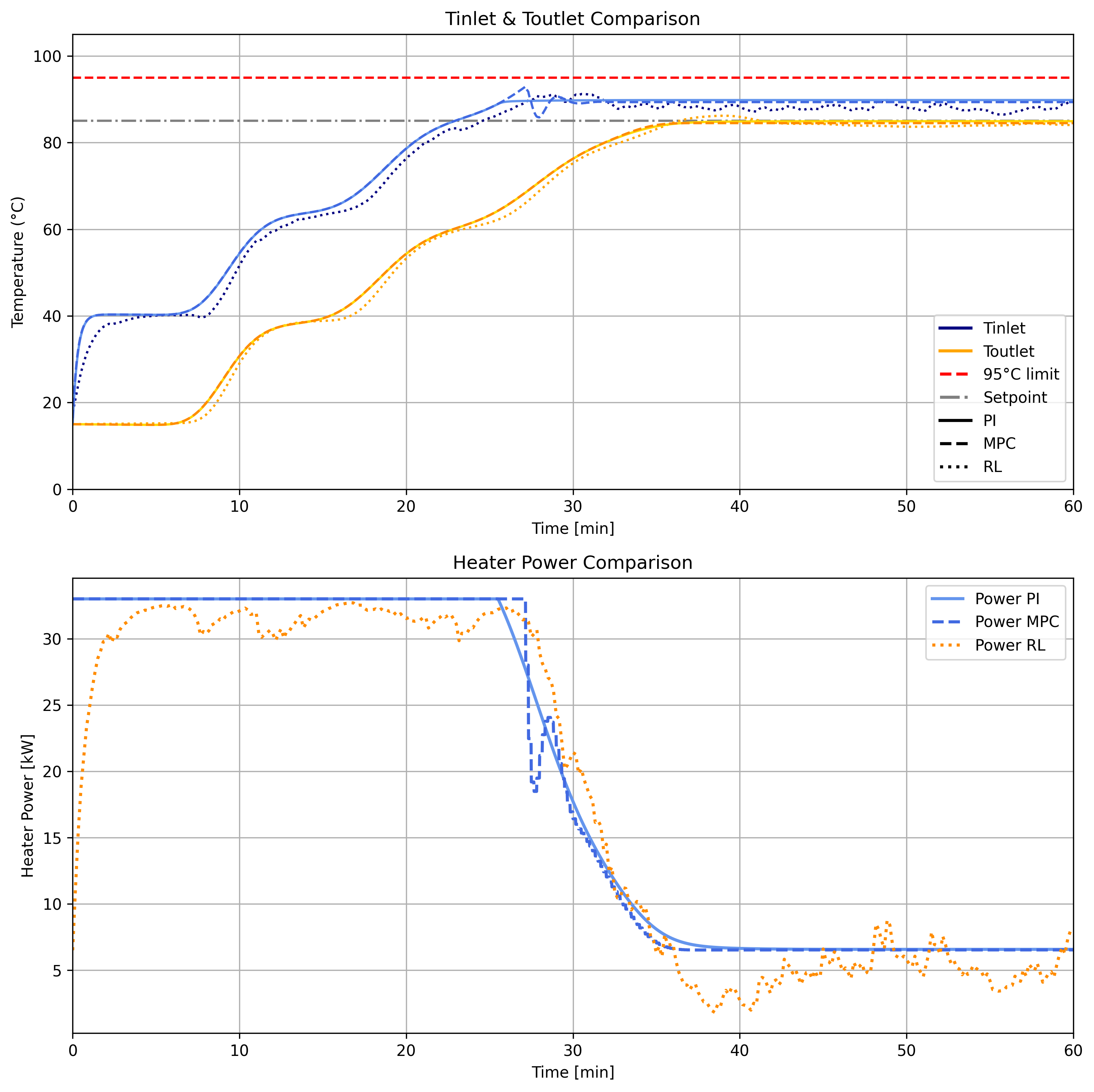
Performance on Step	✅ Excellent	✅ Very good	❌ Shaky
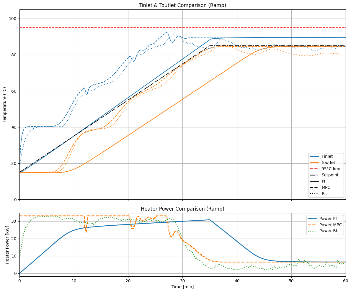
Performance on Ramp	❌ Needs tuning	✅ Very good	❌ Needs training
Security	⚠️ Gain scheduling	✅ Inherent	❌ Must be tested
Complexity/Flexibility	✅ Low	❌ High	⚠️ Retraining
Running Frequency	✅ 1Hz	❌ 0.1Hz	✅ 1Hz

Step input comparison :

Ramp input comparison :

Key Takeaways

• PI control is simple and effective for constant setpoints.

• MPC is robust and handles constraints but is computationally heavy.

• RL is flexible but requires extensive training and validation.

---

📂 Appendix

Parameters

• (x): Position (m)

• (T(x, t)): Temperature (K)

• (u): Fluid velocity (m/s)

• (P): Heater power (W)

• (K): Heat loss coefficient

Simulation Details

• Impact of heat loss coefficient and external temperature:

---

🔧 How to Use

1. Clone the repository.

2. Install all required libraries: numpt, matplotlib, cvxpy, gymnasium, stable-baselines3

3. Run the Jupyter notebook system_tutorial for simulations.

4. Tune parameters for your specific use case.

---

💡 Which Controller Would You Choose?

• For simplicity and constant setpoints: PI control.

• For robustness and constraints: MPC.

• For flexibility and model-free scenarios: RL.

---